INCAR parameter of VASP
1. The bold part is the common control parameters.
2. The annotations are all from the official manual of VASP.
Startparameter for this run:
SYSTEM = Calculation for XXX
NWRITE = 2 # write-flag & timer
PREC = A # normal or accurate (medium, high low for compatibility)
Default: PREC=Normal
The PREC-flag determines the energy cutoff ENCUT, if (and only if) no value is given for ENCUT in the INCAR file. For PREC=Low, ENCUT will be set to the maximal ENMIN value found in the POTCAR files. For PREC=Medium and PREC=Accurate, ENCUT will be set to maximal ENMAX value found on the POTCAR file.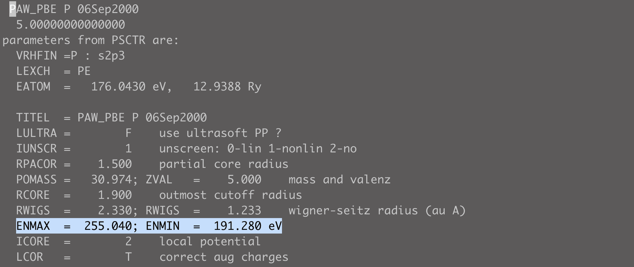
ISTART = 0 # job : 0-new 1-cont 2-samecut
Default: ISTART = 1 if WAVECAR exists, = 0 elseICHARG = 2 # charge: 1-file 2-atom 10-const
Default: ICHARG = 2 if ISTART=0, = 0 else
| ISTART | meaning |
|---|---|
| 0 | Calculate charge density from initial orbitals. |
| 2 | Take superposition of atomic charge densities |
| 11 | To obtain the eigenvalues (for band structure plots) or the DOS for a given charge density read from CHGCAR. The selfconsistent CHGCAR file must be determined beforehand doing by a fully selfconsistent calculation with a k-point grid spanning the entire Brillouin zone. |
| 12 | Non-selfconsistent calculations for a superposition of atomic charge densities. |
ISPIN = 1 # spin polarized calculation?
Default: ISPIN = 1. For ISPIN=1 non spin polarized calculations are performed, whereas for ISPIN=2 spin polarized calculations are performed.LNONCOLLINEAR = F # non collinear calculations
LSORBIT = F # spin-orbit coupling
METAGGA = F # non-selfconsistent MetaGGA calc.
METAGGA = MBJ The modified Becke-Johnson exchange potential in combination with L(S)DA-correlation yields band gaps with an accuracy similar to hybrid functional or GW methods, but computationally less expensive (comparable to standard DFT calculations).
To check whether a particular POTCAR contains this information, type:grep kinetic POTCAR,This should yield at least the following lines:1
2
3kinetic energy density (partial)
kinetic energy-density
mkinetic energy-density pseudized
Electronic Relaxation 1
ENCUT = 550.0 # cutoff, eV
Default: ENCUT = largest ENMAX from POTCAR-fileEDIFF = 1E-04 # stopping-criterion for ELM
Specifies the global break condition for the electronic SC-loop.LREAL = F # real-space projection
Default: LREAL = F, projection done in reciprocal space
- NLSPLINE = F # pline interpolate recip. space projectors
Ionic relaxation
- EDIFFG = -.2E-01 # stopping-criterion for IOM
Default: EDIFFG = EDIFF*10
EDIFFG defines the break condition for the ionic relaxation loop. If EDIFFG is negative, the relaxation will stop if all forces are smaller than |EDIFFG|. This is usually a more convenient setting.
- ISMEAR = 1; SIGMA = 0.2
Determines how the partial occupancies are set for each orbital.
If the cell is too large (or if you use only a single or two k-points) use ISMEAR=0 in combination with a small SIGMA=0.05.
| ISMEAR | meaning |
|---|---|
| -1 | Fermi-smearing |
| 1 | Method of Methfessel-Paxton order. The calculation of phonon frequencies. In metals always use ISMEAR=1 or ISMEAR=2 |
| 0 | Gaussian smearing. Reasonable results in most cases. Insulators |
| -5 | Tetrahedron method with Blöchl corrections (use a Gamma-centered k-mesh. The calculation of the total energy in bulk materials. A good account for the electronic DOS. Semiconductors or insulator |
- NSW = 500 # number of steps for IOM
Default: NSW = 0, sets the maximum number of ionic steps.
- IBRION = 2 # ionic relax: 0-MD 1-quasi-New 2-CG
Default: IBRION= -1 for NSW=0 or NSW=1, = 0 else
| IBRION | meaning |
|---|---|
| 0 | molecular dynamics |
| 2 | for difficult relaxation problems |
| 3 | useful when starting from very bad initial guesses. |
| 5&6 | finite differences to determine the second derivatives |
| 7&8 | density functional perturbation theory to calculate the derivatives. |
- POTIM = 0.1 # no default, must be set by user
In case IBRION=0 (MD) , POTIM specifies the time step in fs. For IBRION=1,2 or 3, POTIM serves as a scaling constant for the forces.
NFREE = 1 # steps in history (QN), initial steepest desc. (CG)
ISIF = 2 # stress and relaxation
ISIF=0 if IBRION=0 (MD), =2 else
Controls whether the stress tensor is calculated.
| ISIF | calculate | calculate | relax | change | change |
|---|---|---|---|---|---|
| force | stress tensor | ions | cell shape | cell volume | |
| 0 | yes | no | yes | no | no |
| 2 | yes | yes | yes | no | no |
| 3 | yes | yes | yes | yes | yes |
| 4 | yes | yes | yes | yes | no |
ISYM = 2 # 0-nonsym 1-usesym 2-fastsym
switch symmetry on (ISYM=1, 2 or 3) or off (ISYM=-1 or 0). For ISYM=2 a more efficient, memory conserving symmetrisation of the charge density is usedTEBEG = 0.0; TEEND = 0.0 temperature during run
TEBEG and TEEND control the temperature during an ab-initio molecular dynamics ruPSTRESS= 0.0 # pullay stress
If the PSTRESS tag is specified VASP will add this stress to to stress tensor, and an energy (unit:kb).
Electronic relaxation 2 (details)
- ALGO = Normal # algorithm
ALGO = Normal selects IALGO = 38 (blocked Davidson iteration scheme)
ALGO = Very_Fast selects IALGO = 48 (RMM-DIIS)
ALGO = Fast:blocked Davidson iteration+RMM-DIIS
- IMIX = 4 # mixing-type and parameters
- AMIX = 0.40; BMIX = 1.00
- AMIX_MAG = 1.60; BMIX_MAG = 1.00
- AMIN = 0.10
- WEIMIN = 0.0010 # energy-eigenvalue tresh-hold
- EBREAK = 0.24E-06 # absolut break condition
- DEPER = 0.30 # relativ break condition
- TIME = 0.40 # timestep for ELM
vdW corrections
IVDW = 0 | 1 | 10 | 11 | 12 | 2 | 20 | 21 | 202 | 4 Default: IVDW = 0
This tag controls whether vdW corrections are calculated or not. If they are calculated IVDW controls how they are calculated
EDFT-disp = EKS-DFT + Edisp, the correction term is computed using some of the available approximate methods
The DFT-D2 method can be activated by setting IVDW=1|10 or by specifying LVDW=.TRUE. (this parameter is obsolete as of VASP.5.3.3)
| IVDW | meaning |
|---|---|
| 0 | no correction |
| 1 / 10 | DFT-D2 method of Grimme (available as of VASP.5.2.11) |
| 11 | zero damping DFT-D3 method of Grimme (available as of VASP.5.3.4) |
| 12 | DFT-D3 method with Becke-Jonson damping (available as of VASP.5.3.4) |
| 2 / 20 | Tkatchenko-Scheffler method (available as of VASP.5.3.3) |
| 21 | Tkatchenko-Scheffler method with iterative Hirshfeld partitioning (available as of VASP.5.3.5) |
| 202 | Many-body dispersion energy method (MBD@rSC) (available as of VASP.5.4.1) |
| 4 | dDsC dispersion correction method (available as of VASP.5.4.1) |
Write flags
LWAVE = F # write WAVECAR
LCHARG = F # write CHGCAR
Determine whether the orbitals (file WAVECAR), the charge densities (file CHGCAR and CHG) are written.LVTOT = F # write LOCPOT, total local potential
Determines whether the total local potential (file LOCPOT ) is written.LVHAR = F # write LOCPOT, Hartree potential only
LELF = F # write electronic localiz. function (ELF)
Create an ELFCAR file or not. This file contains the so-called electron localization function.
NCORE = 4 or NPAR = 4
How many cores work on one orbital.LORBIT = 0 # 0 simple, 1 ext, 2 COOP (PROOUT)
| LORBIT | files written |
|---|---|
| 0 | DOSCAR |
| 10 | DOSCAR and PROCAR file |
| 11 | DOSCAR and lm decomposed PROCAR file |
| 12 | DOSCAR and lm decomposed PROCAR file + phase factors |
Exchange correlation treatment:
- GGA = – # GGA type
| GGA | meaning |
|---|---|
| 91 | Perdew-Wang 91 |
| PE | Perdew-Burke-Ernzerhof (standard PBE) |
| RP | revised Perdew-Burke-Ernzerhof (rPBE) |
| AM | AM05 |
| PS | PBEsol |
- LHFCALC = F ## Hartree Fock is set to
- LHFONE = F Hartree Fock one center treatment
- AEXX = 0.0000 # exact exchange contribution
Linear response parameters
LEPSILON= F # determine dielectric tensor
LRPA = F # only Hartree local field effects (RPA)
Orbital magnetization related:
- ORBITALMAG= F switch on orbital magnetization
- LCHIMAG = F perturbation theory with respect to B field
An example of the INCAR file for structural optimization
1 | System = Structural optimization |
An example of the INCAR file for Self-Consistent Field (SCF) calculation
1 | System = SCF |
An example of the INCAR file for ab initio molecular dynamics (AIMD) calculation with NVT ensemble
1 | SYSTEM = AIMD |
References
[1] https://cms.mpi.univie.ac.at/vasp/guide/node91.html
[2] https://icme.hpc.msstate.edu/mediawiki/images/d/d2/LS14_VASP.pdf
[3] https://www.nersc.gov/assets/Uploads/VASP-tutorial-SurfaceScience.pdf
[4] https://cms.mpi.univie.ac.at/wiki/index.php/Category:Examples
- Blog Link: http://agrh.github.io/2019/07/25/incar/
- Copyright Declaration: The author owns the copyright, please indicate the source reproduced.